

Section contents
Paleoclimate estimation with plant fossils
- Nearest living relative (NLR) methods
- Univariate leaf physiognomic methods
- Climate-Leaf Analysis Multivariate Program (CLAMP)
- Digital leaf physiognomy (DiLP) ←
Digital leaf physiognomy (DiLP)
Digital leaf physiognomy (DiLP) harnesses the power of digital imaging, imaging manipulation, and software to measure irregular shapes. DiLP was developed in work by Huff et al. (2003), Royer et al. (2005), and Peppe et al. (2011, 2018). It is said to yield more accurate results than univariate methods, and to be an improvement over CLAMP analysis in the multivariate realm in that it is more repeatable and objective. It has been applied to a few fossil floras.
DiLP begins with digital imaging of leaves and manipulation of those images to allow for simple and consistent measurements. Note that only the leaf blade (lamina) is used in DiLP calculations. The first step in DiLP is to take digital photographs of the leaves of interest. Ideally, this will be done against a contrasting background to make later manipulation easier.
After images have been made, they can be processed to make the calculations necessary for DiLP simpler:
- Missing or damaged margins must be reconstructed.
- For fossil leaves, the rock matrix must be removed from around the actual leaf specimen.
- The leaf petiole must be removed.
- The leaf image should be processed so that the leaf blade is a solid color. This can be accomplished via different methods (see original papers).
- Any holes in the leaf (due, e.g., to insect damage) should be mended (filled).
Fossil leaves are often fragmentary, so addition methods may be necessary to reconstruct a sufficient number of leaves to create a large enough dataset for DiLF.
ADD INFORMATION
Obviously, best practice dictates that all original and processed images be retained as the raw data for DiLP.
Measurements & variables
Leaf measurements for DiLP MAT and MAP equations1
| Variable (abbreviation) | Definition (units) |
|---|---|
| Blade area (BA) | Area of leaf blade (cm2) |
| Major axis or Major Feret (Maj) | Longest measurable line from edge to edge on leaf blade (cm) |
| Feret's diameter (FD) | Diameter of a circle with the same area as the leaf blade (cm) |
| Feret's diameter ratio (FDR) | Feret's diameter/major axis length (dimensionless) |
| Perimeter (P) | Perimeter of leaf blade (cm) |
| Internal Perimeter (IP) | Perimeter of leaf blade after teeth are removed (cm) |
| Perimeter ratio (PR) | Perimeter/internal perimeter (dimensionless) |
| Number of primary teeth | (count) |
| Number of secondary teeth | (count) |
| Total number of teeth (T) | (count) |
| Standardized tooth count (T:IP) | Number of teeth/internal perimeter (teeth/cm) |
1 After Royer et al. (2005), Peppe et al. (2011, 2018), Glade-Vargas et al. (2018), and Baumgartner et al. (2020). Since the abbreviations for measurements vary among sources, I have chosen a simple set of abbreviations for this discussion.
Leaf blade area (BA)
Leaf blade area is just the surface area of the leaf blade.
Feret's diameter & Feret's diameter ratio (FDR)
Feret's diameter ratio is a ratio of two measurements, Feret's diameter and length of the major leaf axis. Feret's diameter is defined as:
Feret's diameter: measure of an object in a single dimension or direction (length, width, height).
In the case of DiLP, Feret diameter has a specific, distinct meaning:
Feret's diameter (for leaf digital leaf physiognomy): Diameter of a circle with the same area as the leaf blade. This is calculated as 2 × the square root of (leaf area ÷ π).
FD (for DiLF) = 2√(BA ÷ π)
Major axis can be defined as follows:
Major axis (Maj): the longest straight line that connects any two points on the perimeter (edge) of a leaf blade. The major axis is often the length of the leaf blade.
The Feret's diameter ratio is the ratio of the Feret's diameter to the length of the major axis. It is calculated as:
Feret's diameter ratio (FDR) = Feret's diameter of a leaf blade ÷ length of the major axis of a leaf blade.
An example of how to calculate FDR is shown in the figure below. For a leaf with a blade 3.6 cm long and 2.4 cm wide, FDR is calculated as follows:
Major axis = 3.6 cm
BA = 6.8 cm²
Feret's diameter = 2√(6.8 ÷ 3.14) = 2.9 cm
FDR = 2.9 ÷ 3.6 = 0.81
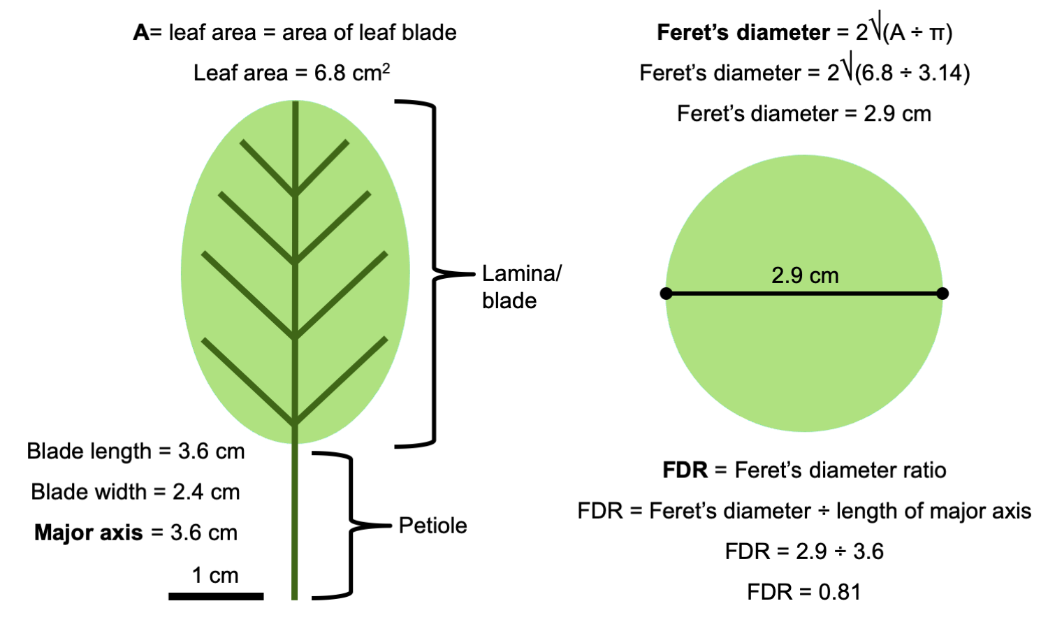
Diagram showing an example calculation for Feret's diameter ratio. The diagram above shows the procedure for determining FDR on a leaf with a blade 3.6 cm long × 2.4 cm wide. Credit: E.J. Hermsen (DEAL).
Perimeter ratio (PR)
Perimeter ratio is the ratio of the leaf perimeter with teeth and without teeth. It is calculated as follows:
Perimeter ratio (PR) = perimeter of leaf ÷ perimeter of leaf with teeth removed.
If a leaf is entire, its perimeter ratio will be one because there are no teeth to be removed. Lobes are not removed in this procedure. For specific instructions for differentiating teeth and lobes, etc., see Royer et al. (2005).
Standardized tooth count (T:IP)
Standardized tooth count is the ratio of the number of leaf teeth to the perimeter of the leaf with the teeth removed.
Standardized tooth count (T:IP) = total number of leaf teeth ÷ perimeter of the leaf with teeth removed.
If the leaf is entire, the T:IP ratio will be zero, because zero divided by any value is zero. If teeth are compound, both primary and secondary teeth are included in the tooth count (see Royer et al., 2005).
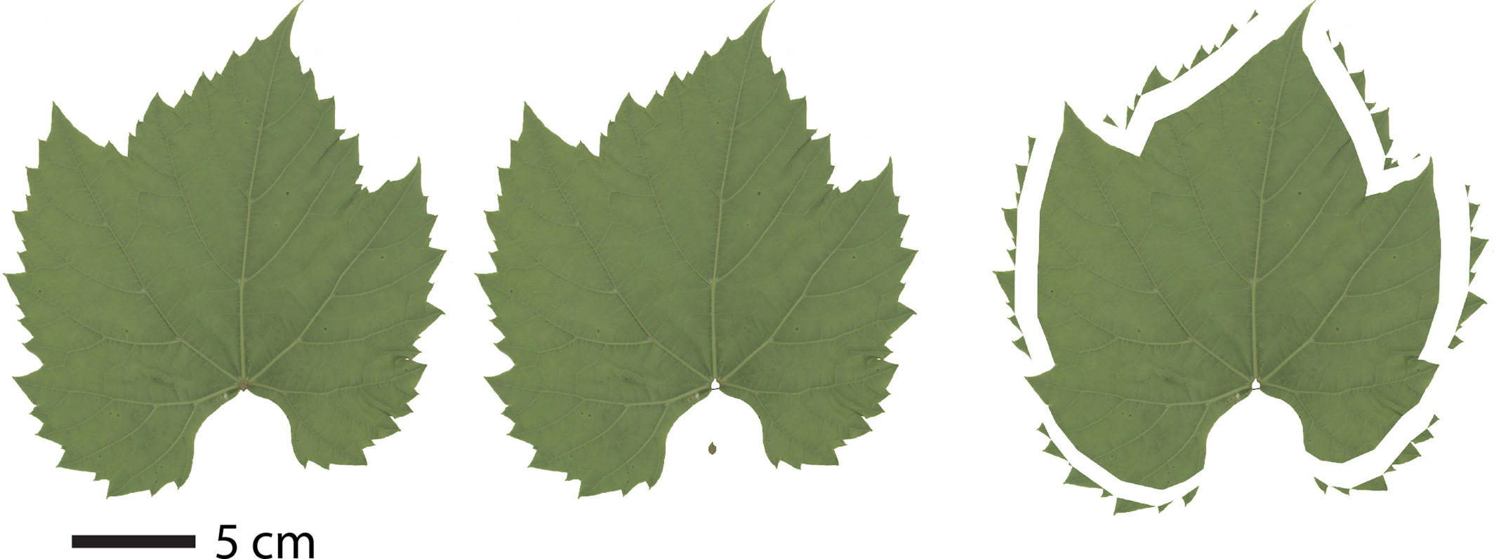
Digital processing of a grape (Vitis) leaf to measure perimeter without teeth. Left: Leaf blade, most of petiole (stalk) removed. Center: Leaf blade, attachment point of petiole removed. Right: Leaf blade, teeth clipped to show the perimeter of leaf without teeth. Credit: Baumgartner et al. (2020) Amer J Bot, fig. 2 (CC BY 4.0).
Determining values for a flora
The above descriptions of measurements and variables describes how to determine values for individual leaves. When using these variables in an equation, however, we need a single number representing each variable to represent a whole flora, so we can plug into an equation. How do we determine these whole-flora values?
Morphotype-type mean values
First, we we need to assign a single value to each variable for each leaf morphotype in a flora. The first step in doing this is, of course, to sort leaf specimens into morphotype categories. After that, individual leaves can be digitized, measured, and scored. Scoring is just making a table of measurements and calculations that describe each leaf. An exemplar of at least one leaf representing each morphotype in a flora should be scored, if possible; ideally, more than one leaf will be scored per morphotype. Note that leaves can be scored for some values even if not all values can be measured. Once leaves are scored for features that can be directly measured or observed, variables (like Feret's diameter and Feret's diameter ratio) can be calculated for each leaf.
Once you have made a table with the measurements and calculations for each leaf, you can determine morphotype-mean values for each morphotype. In order to do this, simply find the mean (average) of each measurement and variable for the set of leaves in each morphotype. If a scored leaf lacks a particular measurement or variable, leave it out of the average for the affected measurement or variable. If only one leaf was scored a morphotype, then its scores are the values for the morphotype.
Site-mean values
Finally, morphotype-mean values must be used to compute site-mean values. A site-mean value for a given variable is just the mean (average) of the morphotype-mean values for that variable. The site-mean values are the values actually used in the equations for mean annual temperature (MAT) and mean annual precipitation (MAP) given below.
Example table of leaf morphotype scores, calculated morphotype means, and calculated site means for leaf variables2
| Margin | Leaf blade area (BA), cm2 | Major axis length, cm | Total number of teeth (T) | Internal perimeter (IP), cm | Feret's diameter (FD) | Feret's diameter ratio (FDR) | Standarized tooth count (T:IP), teeth/cm | |
|---|---|---|---|---|---|---|---|---|
| Morphotype A, leaf 1 | toothed | 50.5 | 10.3 | 10.0 | 20.6 | 8.0 | 0.8 | 0.5 |
| Morphotype A, leaf 2 | toothed | 32.2 | 8.4 | 6.0 | 12.1 | 6.4 | 0.8 | 0.5 |
| Morphotype A, leaf 3 | toothed | 46.0 | 8.0 | 8.0 | 20.0 | 7.7 | 1.0 | 0.4 |
| Morphotype A mean | toothed | 42.9 | 8.9 | 8.0 | 17.6 | 7.4 | 0.8 | 0.5 |
| Morphotype B, leaf 1 | untoothed | 54.7 | 12.3 | 0.0 | 21.0 | 8.3 | 0.7 | |
| Morphotype B mean | untoothed | 54.7 | 12.3 | 0.0 | 21.0 | 8.3 | 0.7 | |
| Morphotype C, leaf 1 | toothed | 30.5 | 10.2 | 12.0 | 24.5 | 6.2 | 0.6 | 0.5 |
| Morphotype C, leaf 2 | toothed | 21.6 | 10.0 | 17.3 | 5.2 | 0.6 | ||
| Morphotype C, leaf 3 | toothed | 25.6 | 10.0 | 5.7 | ||||
| Morphotype C mean | toothed | 25.9 | 10.2 | 10.7 | 20.9 | 5.7 | 0.6 | 0.5 |
| Site mean | 41.2 | 10.5 | 6.2 | 19.8 | 7.1 | 0.7 | 0.5 | |
| Percent entire (untoothed), flora (E) | 33.3% |
2 The above table shows a hypothetical example of scoring of leaf morphotypes for DiLP analysis of MAT; only selected characters are shown in order to simplify the example. Individual leaves in each morphotype category are scored separately. The scores for each morphotype are averaged to produced a morphotype-mean value for each variable. Finally, the morphotype-mean values are averaged to produce a site-mean value for each variable.
Mean annual temperature
The mean annual temperature (MAT) equation for DiLF was proposed be Peppe et al. (2011). The equation is as follows:
MAT = 0.21E + 42.296(FDR) - 2.609(T:IP) - 16.004
Where:
MAT = mean annual temperature, the variable being calculated.
E = percent of species with entire (in this analysis, meaning untoothed) margins.
This value is calculated as follows: number of woody dicot species with entire-margined (untoothed) leaves ÷ total number of woody dicot species × 100
FDR = Feret's diameter ratio.
This value is the site-mean FDR. See above for calculation.
T:IP = number of teeth to internal leaf perimeter.
This value is the site-mean T:IP. The entire-margined species may be omitted from the site-mean T:IP. See above for calculation.
Origin of the equation
The equation above is based on an equation from multiple regression analysis. The general multiple regression equation looks like this:
y = b1x1 + b2x2 + b3x3 + a
The purpose of multiple regression analysis is to estimate a dependent variable (y) from a set of independent variables (x1, x2, x3, etc.). In the equation above, the dependent variable (y) that we are estimating is mean annual temperature (MAT). The independent variables (x1, x2, x3) that we are using to estimate MAT are:
x1 = E, the percent entire-margined woody dicot species in a given flora.
x2 = FDR, the site-mean Fermet's diameter ratio.
x3 = T:IP, the site-mean standardized tooth count (number of teeth ÷ internal leaf perimeter in cm).
The numbers preceding each independent variable (b1, b2, b3) are regression coefficients (regression weights) for each of the independent variables. Regression coefficients quantify the correlation in change between each independent variable and the dependent variable; they are equivalent to slopes for each of the independent variables. Remember:
Slope of a line = (change in y) ÷ (change in x)
For example, in the equation above, the regression coefficient for percent entire-margined woody dicot species (x1 or E) is 0.21. Thus, there is a 0.21ºC change in mean annual temperature (MAT or y) for every 1% change in entire-margined woody dicot species (E) provided that the other independent variables (FDR and T:IP) do not change. Remember, the DiLP equation is balancing information from three independent variables (E, FDR, and T:IP) to predict one dependent variable (MAT). Thus, the regression coefficients help to determine the weights given to each of the independent variables.
Finally, a is a constant equivalent to the y-intercept (y=0). In the above equation, it is -16.004. Thus, when y = 0:
0.21E + 42.296(FDR) - 2.609(T:IP) = 16.004
Mean annual precipitation
Mean annual precipitation can be calculated using the following formula:
ln(MAP) = 0.298ln(BA*100) - 2.71ln(PR) + 0.279ln(T:IP) + 3.033
Where:
ln = natural logarithm.
ln(MAP) = natural logarithm of mean annual precipitation (MAP).
ln(BA in mm2) = site mean for the natural logarithm of leaf blade area in mm.
Note: BA in mm2 = 100 × (BA in cm2)
ln(PR) = site mean for the natural logarithm of perimeter ratio (perimeter ÷ internal perimeter).
ln(T:IP) = site mean for the natural logarithm of standardized tooth count (teeth per cm of internal perimeter).
Make note of the fact that blade area is in millimeters squared (mm2), whereas standardized tooth count is expressed as teeth/cm (cm-1).
The DiLP MAP equation has the same structure as the equation above, except that we are solving for the natural log (ln) of mean annual precipitation (MAP), rather than MAP directly. In order to calculate MAP, the equation must be solved for ln(MAP). Then, the following must be calculated.
MAP = eln(MAP)
Where:
e = 2.718281828459 . . .
The number represented by e is a mathematical constant, like pi (π, approximately 3.14).
References & further reading
Note: Free full text is made available by the publisher for items marked with a green asterisk.
Academic articles & book chapters
Allen, S.E., A.J. Lowe, D.J. Peppe, and Herbert W. Meyer. 2020. Paleoclimate and paleoecology of the latest Eocene Florissant flora (Central Colorado, USA). Palaeogeography, Palaeoclimatology, and Paleoecology. https://doi.org/10.1016/j.palaeo.2020.109678
* Baumgartner, A., M. Donahoo, D.H. Chitwood, D.J. Peppe. 2020. The influences of environmental change and development on leaf shape in Vitis. American Journal of Botany. https://doi.org/10.1002/ajb2.1460
* Glade-Vargas, N., L.F. Hinojosa, and M. Leppe. 2018. Evolution of climatic related leaf traits in the family Nothofagaceae. Frontiers in Plant Science 9: 1073. https://doi.org/10.3389/fpls.2018.01073
Huff, P.M., P. Wilf, and E.J. Azumah. 2003. Digital future for paleoclimate estimation from fossil leaves? Preliminary results. PALAIOS 18: 266–274. https://doi.org/10.1669/0883-1351(2003)018<0266:DFFPEF>2.0.CO;2
Lowe, A.J., D.R. Greenwood, C.K. West, J.M. Galloway, M. Sudermann, and T. Reichgelt. 2018. Plant community ecology and climate on an upland volcanic landscape during the Early Eocene Climatic Optimum: McAbee Fossil Beds, British Columbia, Canada. Palaeogeography, Palaeoclimatology, Palaeoecology 511: 433–448. https://doi.org/10.1016/j.palaeo.2018.09.010
Peppe, D.J., A. Baumgartner, A. Flynn, and B. Blonder. 2018. Reconstructing paleoclimate and paleoecology using fossil leaves. Pp. 289–317 in D.A. Croft, D.F. Su, and S.W. Simpson, eds. Methods in Paleoecology: Reconstructing Cenozoic Terrestrial Environments. Springer Nature Switzerland AG, Switzerland. https://doi.org/10.1007/978-3-319-94265-0_13
* Peppe, D.J., D.L. Royer, B. Cariglino, S.Y. Oliver, S. Newman, E. Leight, G. Enikolopov, M. Fernandez-Burgos, F. Herrera, J.M. Adams, E. Correa, E.D. Currano, J.M. Erickson, L.F. Hinojosa, J.W. Hoganson, A. Iglesias, C.A. Jaramillo, K.R. Johnson, G.J. Jordan, N.J.B. Kraft, E.C. Lovelock, C.H. Lusk, Ü. Niinemets, J. Peñuelas, G. Rapson, S.L. Wing, I.J. Wright. 2011. Sensitivity of leaf size and shape to climate: global patterns and paleoclimatic applications. New Phytologist 190: 724–739. https://doi.org/10.1111/j.1469-8137.2010.03615.x
Royer, D.L. 2012. Climate reconstruction from leaf size and shape: New developments and challenges. Pp. 195–212 in L.C. Ivany and B.T. Huber, eds. Reconstructing Earth's Deep-Time Climate—The State of the Art 2012 (Paleontology Society Short Course, November 3, 2012). The Paleontological Society Papers 18. https://doi.org/10.1017/S1089332600002618
* Royer, D.L., P. Wilf, D.A. Janesko, E.A. Kowalski, and D.L. Dilcher. 2005. Correlations of climate and plant ecology to leaf size and shape: potential proxies for the fossil record. American Journal of Botany 92: 1141–1151. https://doi.org/10.3732/ajb.92.7.1141
Content usage
Usage of text and images created for DEAL: Text on this page was written by Elizabeth J. Hermsen. Original written content created by E.J. Hermsen for the Digital Encyclopedia of Ancient Life that appears on this page is licensed under a Creative Commons Attribution-NonCommercial-ShareAlike 4.0 International License. Original images created by E.J. Hermsen are also licensed under Creative Commons Attribution-NonCommercial-ShareAlike 4.0 International License.
Content sourced from other websites: Attribution, source webpage, and licensing information or terms of use are indicated for images sourced from other websites in the figure caption below the relevant image. See original sources for further details. Attribution and source webpage are indicated for embedded videos. See original sources for terms of use. Reproduction of an image or video on this page does not imply endorsement by the author, creator, source website, publisher, and/or copyright holder.
Adapted images. Images that have been adapted or remixed for DEAL (e.g., labelled images, multipanel figures) are governed by the terms of the original image license(s) covering attribution, general reuse, and commercial reuse. DEAL places no further restrictions above or beyond those of the original creator(s) and/or copyright holder(s) on adapted images, although we ask that you credit DEAL if reusing an adapted image from the DEAL website. Please note that some DEAL figures may only be reused with permission of the creator(s) or copyright holder(s) of the original images. Consult the individual image credits for further details.
First released XX Month 2020; last updated XX Month 2020.