


Section contents:
- Introduction & Methods (previous section)
- Live-dead Mismatch as a Conservation Tool
- Case Studies & Looking to the Future (next section)
Feature Image: Photograph of the sea floor in Long Island Sound, New York and Connecticut, from USGS survey 2018-018-FA. Photograph by Ackerman, S.D., Huntley, E.C., Blackwood, D.S., Babb, I.G., Zajac, R.N., Conroy, C.W., Auster, P.J., Schneeberger, C.L., and Walton, O.L., 2020, Sea-floor sediment and imagery data collected in Long Island Sound, Connecticut and New York, 2017 and 2018: U.S. Geological Survey data release, https://doi.org/10.5066/
Live-dead Mismatch as a Conservation Tool
Research has shown that death assemblages provide a good representation of the living assemblage (Kidwell, 2009); therefore, we expect the species within the living and death assemblages to match under normal conditions. This does not necessarily indicate ideal ‘healthy’ or ‘natural’ environmental conditions, but rather that there has not been a recent change in conditions that would be reflected in the death assemblage. However, if the species composition (or other ecological attribute) between the living and death assemblages differs, there has likely been a recent change in environmental conditions that caused a mismatch.
Environmental stressors are direct and indirect drivers that lead to biodiversity loss and ecosystem degradation, which can often help explain the mismatch observed between the living and death assemblages. The most common anthropogenic environmental stressors are habitat change, climate change, overexploitation, the spread of non-native species, and pollution. Each of these stressors may act independently or sometimes interact simultaneously resulting in a mismatch between the living and death assemblages.
Live-dead studies either begin with data collection or previous knowledge about the history of an environmental stressor or change in species within a local area. In the next section, we walk through a hypothetical example of how a live-dead mismatch study can be conducted.
Hypothetical Example: Seagrass in Barnegat Bay, New Jersey
Background:
Over the past 25 years, seagrass habitat has been disappearing in Barnegat Bay, New Jersey from a combination of multiple stressors, including harmful algal blooms that reduce light availability, and increased boating activity that may be shredding existing seagrass beds (known as boat scarring). Mapped surveys from the late-1960s and late-1970s have been used as baselines for both documenting the loss of seagrass (primarily eelgrass, Zostrea marina) populations in Barnegat Bay and for establishing areas for seagrass restoration (Barnegat Bay Partnership, 2024; Kennish et al., 2007; Lathrop et al., 2001). However, seagrass populations have likely been in decline since the mass wasting disease epidemic of the 1930s, which affected many seagrass populations along the Atlantic coast of the United States (Campanella et al. 2023). Without survey records prior to 1968, it is unknown how much seagrass habitat existed before the 1930s wasting disease epidemic and therefore it is unknown whether the 1960-1970 baseline represents an already degraded condition (referred to as a shifted baseline).
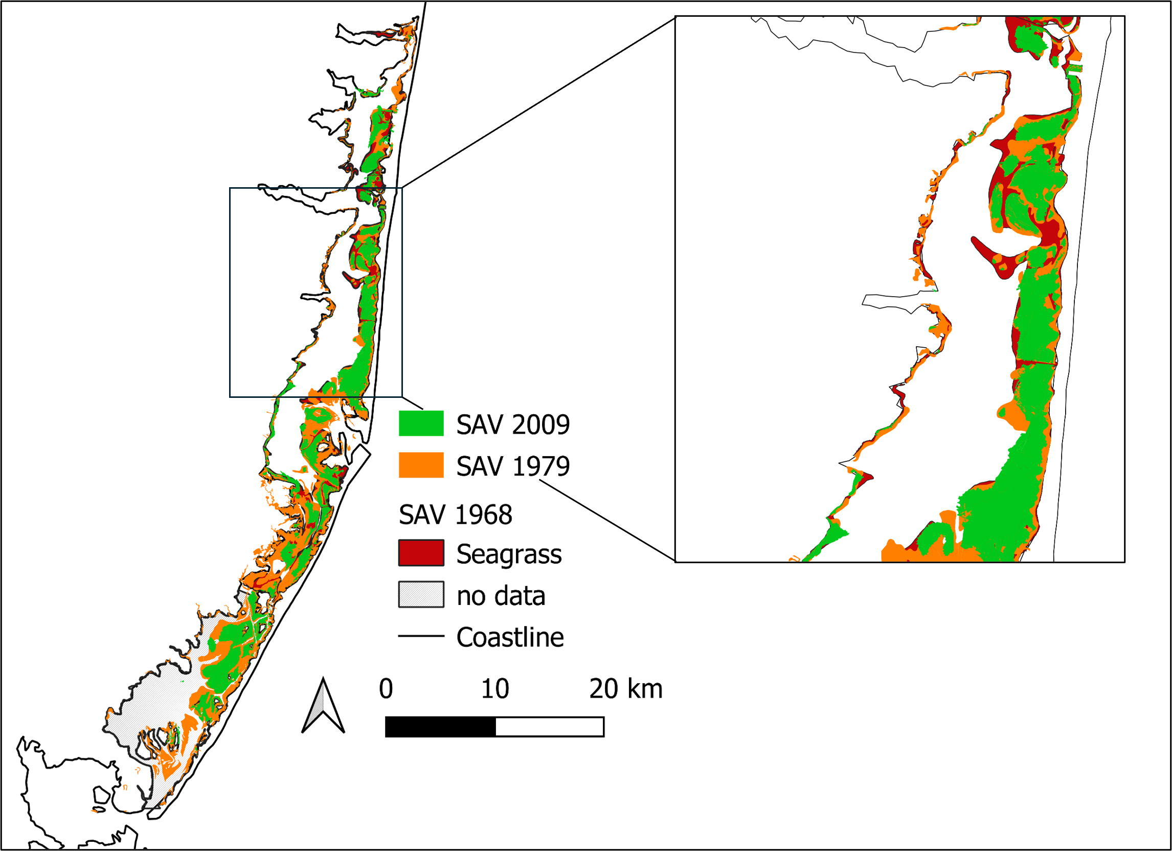
Seagrass in Barnegat Bay. Map of the spatial distribution of submerged aquatic vegetation (SAV) in Barnegat Bay, New Jersey in 1968 (red), 1979 (orange), and 2009 (green). SAV data from Grant F. Walton Center for Remote Sensing and Spatial Analysis (CRSSA), Rutgers University. U.S. Coastline shapefile from National Atlas of the United States, U.S. Geological Survey, 201403. Figure by Matthew J. Pruden.
Questions:
Was the historic (pre-1960s) spatial extent of seagrass beds greater than the 1960-1970 survey baselines? Do the 1960-1970 data represent a shifted baseline?
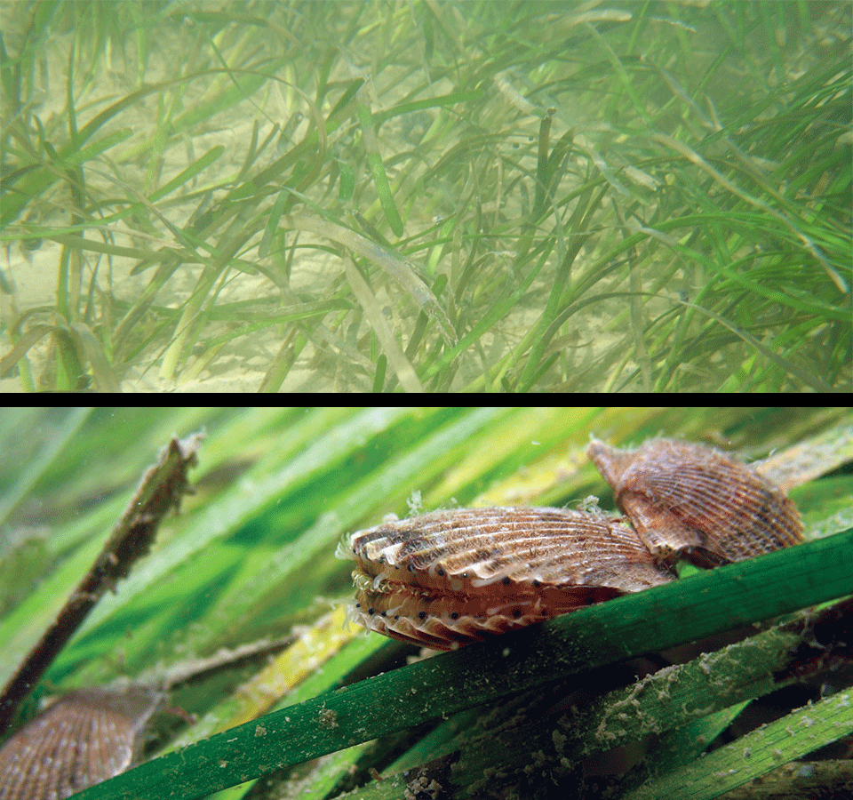
Top: An eelgrass (Zostera marina) meadow. Photograph by Claude Nozères (Wikimedia Commons; Creative Commons Attribution-Share Alike 4.0 International license). Bottom: Bay scallops (Argopecten irradians) in an eelgrass bed. Approximate scallop size in image ~1cm or less, photograph by Bob Orth, Submerged Aquatic Vegetation Program, Virginia Institute of Marine Science (Creative Commons BY 2.0).
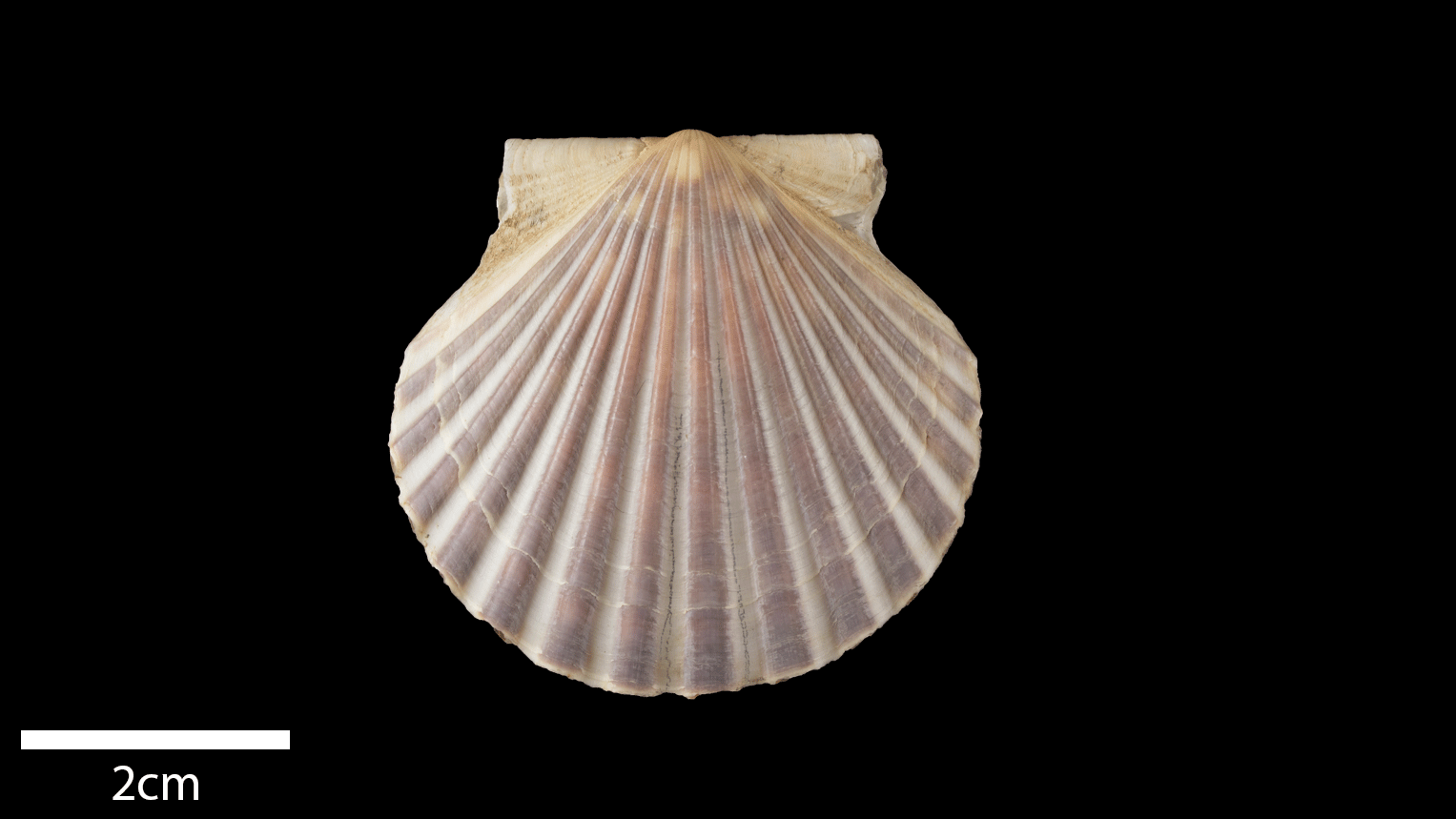
Photograph of an Atlantic Bay Scallop (Argopecten irradians: PRI 108740). Specimen is from the collections of the Paleontological Research Institution, Ithaca, New York. Photograph by Jaleigh Q. Goben.
How Could the Samples be Collected?
To determine whether the historic spatial extent of seagrass extended beyond the 1960-1970 baseline, live-dead samples could be collected from: 1) areas of known seagrass loss; 2) areas that could have supported seagrass (based on historical records of depth and sediment type because seagrass has specific tolerances for environmental conditions), but where no seagrass beds have been officially documented; and 3) in areas that still have seagrass to identify which species are likely to be preserved in a seagrass death assemblage. Molluscan species commonly associated with seagrass beds in Barnegat Bay include bay scallops (Argopecten irradians), cerith snails (e.g., Bittiolum alternatum) and the rough periwinkle (Littorina saxatilis). To minimize the impact of sampling volume on the analysis, all samples could be collected using the same method with a predetermined volume, such as a 25 cm diameter push core. All samples could then be sieved using a 1 mm mesh sieve (see Box 1).
The number of live-dead samples needed depends on the specific areas of interest as well as feasibility given time and financial constraints. For this project, collecting dozens of samples across the entirety of Barnegat Bay would be ideal. This might include mapping out a grid across Barnegat Bay and randomly selecting sample sites of known or expected seagrass presence. The more samples, the more statistically robust the analysis would be.
What Types of Analyses Could be Run?
First, because the goal of this hypothetical study is to identify the historic spatial extent of seagrass beds, we could identify all taxa in both the living and death assemblages to the lowest possible taxonomic level (i.e., species) and compare the taxonomic similarities and rank abundances between the living and death assemblages (see Box 2 for possible metrics). Comparisons could also be made between the samples taken in areas of known seagrass loss to areas with no documented seagrass beds to assess whether the live-dead mismatch is consistent between the two areas. It would also be important to radiocarbon date the death assemblages to check whether they pre-date the 1960s/70s surveys, preferably back to at least the 1930s.
What Could Potential Results and Interpretations Look Like?
If the areas without seagrass beds did have historic seagrass beds (pre-1960s), we would expect a mismatch in both taxonomic similarity and rank abundance between the death and living assemblages, similar to the samples taken from areas of known seagrass loss. The death assemblages would have higher abundances of seagrass-associated species, such as bay scallops. In contrast, the living assemblages would be dominated by sand-associated species. These results might indicate that the spatial extent of seagrass beds in Barnegat Bay was greater than the 1960-1970 baseline, and would indicate a need to reevaluate the current restoration targets and expand the list of potential restoration sites.
If the area sampled did not have historic seagrass beds or did not pre-date the 1960s, then we would expect greater live-dead matching in taxonomic similarity and rank abundance. Thus, depending on the age of the death assemblages, we would conclude that: 1) If the death assemblages pre-date the 1960s, then the 1960-1970 baseline may be adequate for designating areas for seagrass restoration; or 2) If the death assemblages do not pre-date the 1960s, then the death assemblages are not old enough to determine if the spatial extent of seagrass beds was greater in the past and we may have to dig deeper to access older samples.
Alternative Explanations for Mismatch
If anthropogenic change can not clearly explain a live-dead mismatch, there are several alternative reasons worth investigating, which we outline below following Kidwell (2013):
1. Undersampling: Differences in volume (even when using the same type of gear) or the number of samples could result in misleading comparisons between the living and death assemblage (see Box 1). For example, undersampling the living assemblage could exaggerate the differences in species abundance or diversity.
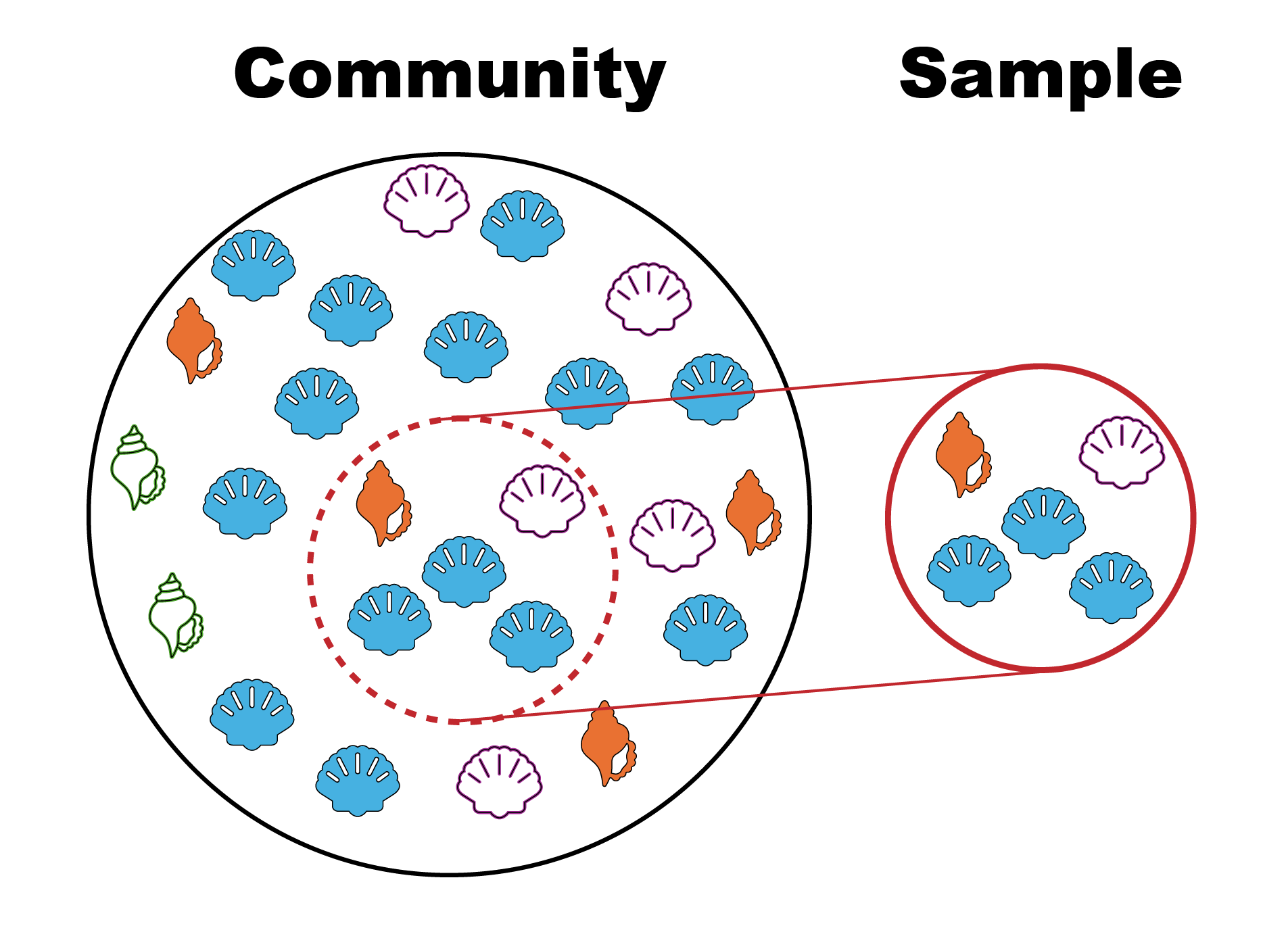
Community vs Sample. The circle on the left represents all species within a community, whereas the circle on the right represents a sample of species from the community. Sometimes a sample from a community does not sample the true number of species found in a given area. Graphic by Jaleigh Q. Goben is licensed under a Creative Commons Attribution-ShareAlike 4.0 International License.
2. Collection Bias: Different sampling gear (e.g., dredging vs. box-core sampling) could lead to a death assemblage bias by not sampling environments in the same way. For example, mobile species are more likely to be collected using a dredge than a box-core.
3. Time-averaging: Time-averaging can result in the accumulation of species that are relatively rare in the living assemblage, resulting in greater live-dead mismatch. Therefore, if the death assemblage contains a high number of rare species that are absent in the living assemblage, then the live-dead mismatch may be attributable to a high degree of time-averaging. Alternatively, the presence of rare species unique to the living assemblage may indicate very low degrees of time-averaging, which can also result in greater live-dead mismatch. It is important to have an estimate of the degree of time-averaging to identify how much it could be affecting mismatch.
4. Taphonomic Bias: Preservation potential is an important determining factor as to whether a species will be represented in both the living and death assemblages. If a species has low preservation potential, meaning it lacks hard parts or is fragile (e.g., thinner, smaller shell), it will be less likely to preserve within the death assemblage, which may lead to a species from the living assemblage that is missing in the death assemblage. If a species from the death assemblage is missing from the living assemblage, it could indicate a local disturbance (e.g., a storm, tides, currents, etc.) mixed up the sediments, reworked deeper, older material upward closer to the surface, or transported shells into or out of the area. Smaller species may be more likely to wash away during a disturbance or through the sample sieving process. If a sample is not thoroughly washed, small shells can be retained within larger shells and result in a mismatch. Other organisms, like predators or hermit crabs that are known to inhabit dead snail shells, could also move shells across locations. To ensure a mismatch is not the result of disturbance or taphonomic bias, it is important to compare living and death assemblages in nearby areas within similar environments and identify any patterns in species presence or preservation.
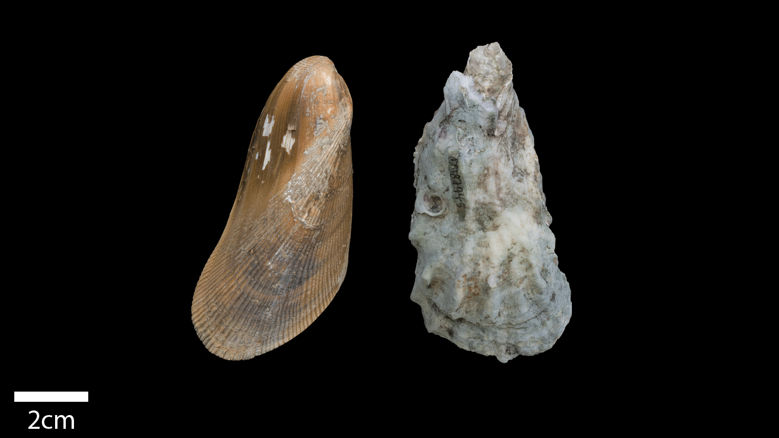
Left: The ribbed mussel (Geukensia demissa; PRI 87782). Mussels have a low preservation potential due to their thin, fragile shells that are often fragmented within a death assemblage. Right: An Eastern Oyster (Crassostrea virginica; PRI 87945). Oysters have a high preservation potential due to their thick, sturdy shells and are often well-preserved within a death assemblage. Specimens are from the collections of the Paleontological Research Institution, Ithaca, New York. Photographs by Jaleigh Q. Goben.
5. ‘Non-human’ Ecological Change: If a species is unique to either the living or death assemblage, it could signal a change in the local environment resulting in species turnover or migration shifts into or out of an area. Natural (non-human) changes in the local environment could lead to a new species colonizing the area, which would only be recorded within the living assemblage. Local changes could also lead to a species no longer being able to flourish in the area, resulting in certain species only present within the death assemblage. Understanding local shifts in species ranges or species characteristics is important to compare with local proxy records for environmental shifts in conditions like temperature, salinity, precipitation, etc. to indicate if a mismatch could result from changes in the environment or local ecology.
If these sampling and natural processes have been checked without a clear indicator leading to a mismatch between the living and death assemblages, then environmental stressors resulting from human impacts are the more likely cause.
References & Further Reading:
Campanella, J. J., P. A. Bologna, A. J. Alhaddad, E. A. Medina, A. Ackerman, J. Kopell, N. R. Ortiz, and M. H. T. Theodore. 2023. Improvement of genetic health and diversity of Zostera marina (eelgrass) in Barnegat Bay, New Jersey ten years after Hurricane Sandy: Support for the “storm stimulus” hypothesis. Aquatic Botany, 189: 103707.
Dietl, G.P., Kidwell, S.M., Brenner, M., Burney, D.A., Flessa, K.W., Jackson, S.T., and P.L. Koch. (2015). Conservation paleobiology: Leveraging knowledge of the past to inform conservation and restoration. Annual Reviews of Earth and Planetary Science, 43: 79-103.
Kennish, M.J. 2007. Barnegat Bay-Little Egg Harbor Estuary: Ecosystem Condition and Recommendations. Rutgers University, Institute of Marine and Coastal Sciences.
Kidwell, S. M., G. P. Dietl, and K. W. Flessa. 2009. Evaluating human modification of shallow marine ecosystems: mismatch in composition of molluscan living and time-averaged death assemblages. Paleontological Society Papers, 15: 113-139.
Kidwell, S. M. 2013. Time‐averaging and fidelity of modern death assemblages: building a taphonomic foundation for conservation palaeobiology. Palaeontology, 56(3): 487-522.
Lathrop, R. G., R. M. Styles, S. P. Seitzinger, and J. A. Bognar. 2001. Use of GIS mapping and modeling approaches to examine the spatial distribution of seagrasses in Barnegat Bay, New Jersey. Estuaries, 24: 904-916.