


Chapter by:
Jaleigh Q. Goben, Mathew J. Pruden, Bridget T. Kelly, and Gregory P. Dietl. Paleontological Research Institution, Ithaca, NY.
Citation:
Goben, J.Q., Pruden, M.J., Kelly, B.T., and G.P. Dietl. 2025. Live-Dead Analysis in Conservation Paleobiology. In: The Digital Encyclopedia of Ancient Life. https://www.digitalatlasofancientlife.org/learn/conservation-paleobiology/live-dead-analysis
Chapter last updated February 4, 2025.
Section contents:
- Introduction & Methods
- Background
- Sample Collection
- Analytical Comparisons
- Live-dead Mismatch as a Conservation Tool
- Case Studies & Looking to the Future
Related pages/background reading:
Feature image: Photograph of slipper shells (Crepidula sp.) along the coast of Long Island Sound. Photograph by Matthew J. Pruden.
Content usage
Usage of text and images created for DEAL: Original written content and original images created by the authors for the Digital Encyclopedia of Ancient Life that appears on this page is licensed under a Creative Commons Attribution-NonCommercial-ShareAlike 4.0 International License.
Content sourced from other websites: Attribution, source webpage, and licensing information or terms of use are indicated for images sourced from other websites in the figure caption below the relevant image. See original sources for further details. Attribution and source webpage are indicated for embedded videos. See original sources for terms of use. Reproduction of an image or video on this page does not imply endorsement by the author, creator, source website, publisher, and/or copyright holder.
Adapted images. Images that have been adapted or remixed for DEAL (e.g., labelled images, multipanel figures) are governed by the terms of the original image license(s) covering attribution, general reuse, and commercial reuse. DEAL places no further restrictions above or beyond those of the original creator(s) and/or copyright holder(s) on adapted images, although we ask that you credit DEAL if reusing an adapted image from the DEAL website. Please note that some DEAL figures may only be reused with permission of the creator(s) or copyright holder(s) of the original images. Consult the individual image credits for further details.
Funding
The material in this chapter is based upon work supported by the National Science Foundation under grant number DEB 2101814 (PI: G. Dietl). Any opinions, findings, and conclusions or recommendations expressed in this material are those of the authors and do not necessarily reflect the view of the National Science Foundation.
Background
Live-dead analysis is a common conservation paleobiology tool that is frequently applied in shallow marine soft-sediment environments to compare living and death assemblages. A living assemblage represents the organisms currently living at a location. A death assemblage is an accumulation of recently dead organisms from the living assemblage with easily preserved hard parts (e.g., clam and snail shells). Over time, dead remains from different years become mixed together resulting in a time-averaged assemblage. This means shells within a death assemblage may not have been alive at the same time.
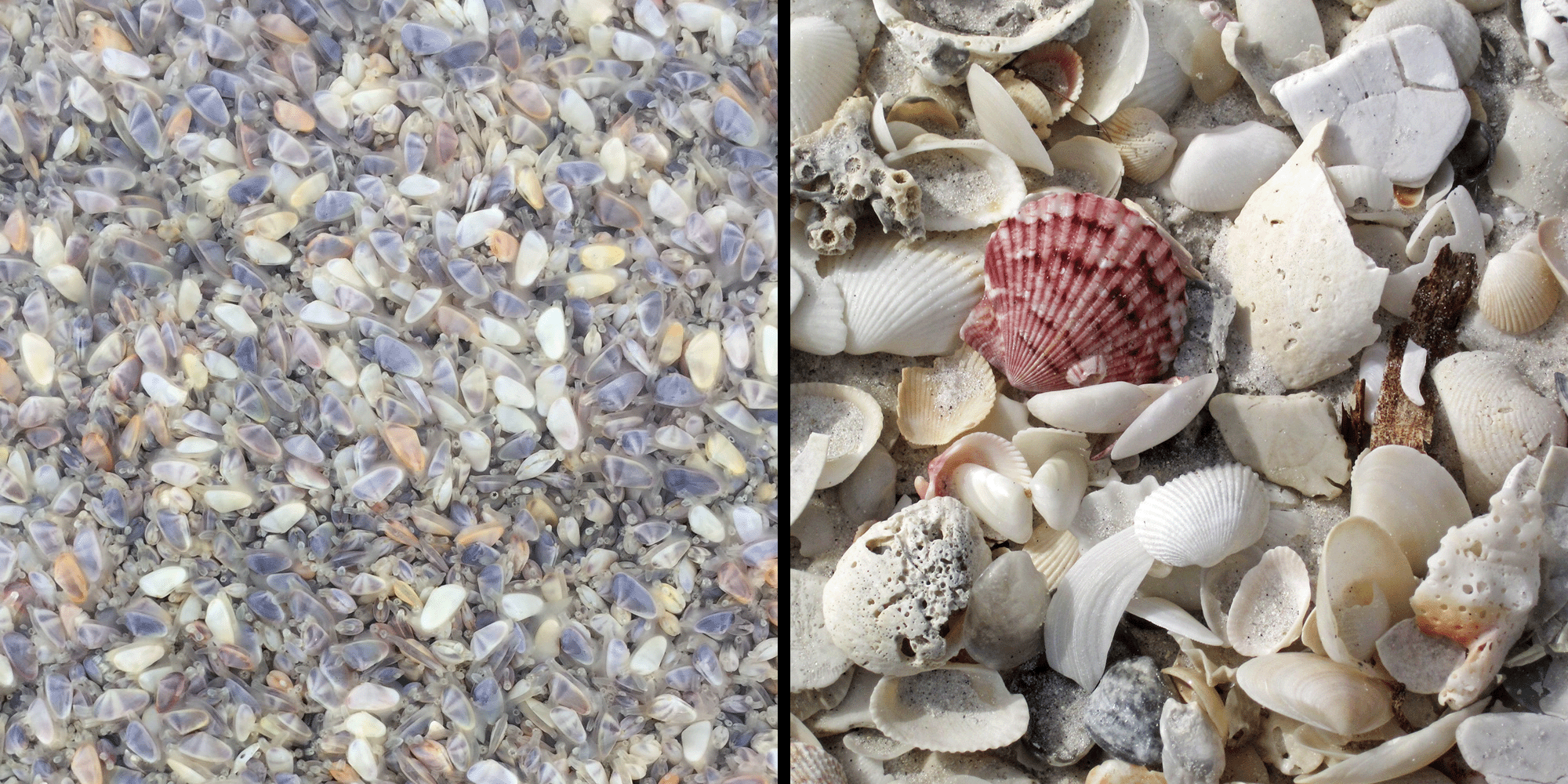
Left: Living assemblage of coquina clams (Donax variabilis) from Stone Harbor, New Jersey. Photograph by Greg Dietl. Right: Beach death assemblage including coquina clams. Photograph by James St. John (Flickr; Creative Commons BY 2.0).
The gradual way death assemblages form results in a ‘lag effect’ of species preservation. If the living assemblage or environment changes, it will take time for the death assemblage to reflect the change, resulting in a mismatch. By comparing species between living and death assemblages, conservation paleobiologists can determine if the community is changing over time and identify clues as to which potential environmental stressors (e.g., pollution, overexploitation) could be causing that change.
Although there are a variety of environments and species that can be applied in live-dead analyses, here we focus on the most common among macroinvertebrates: mollusks (e.g., snails, clams) within shallow, marine, soft-sediment environments.
Sample Collection
Samples of living and death assemblages are collected at the same time using a variety of sampling gear with predetermined volumes, such as Van Veen grabs and small box-cores. The samples are collected at the same time because death assemblages form directly from the molluscan community living within the uppermost sedimentary record (5-20cm). Once the samples have been collected, they are rinsed, sieved to a specific size, sorted, and the taxa within the samples are identified.

Van Veen grab. Photograph by Hans Hillewaert (Wikimedia Commons; Creative Commons Attribution-Share Alike 4.0 International license).
Left: Death assemblage from a Van Veen grab sample collected as part of the 2020 Environmental Protection Agency National Coastal Conditions Assessment Long Island Sound Embayment Intensification. Photograph by Kyle Dayton. Right: Sorting a death assemblage sample and identifying species. Photograph by Kiera Crowley.
Box 1. Importance of standardized volumes and sieve size.
Standardized Volumes:
The number of species collected and their associated abundances are impacted by the volume of material sampled. More volume means a larger sample size and therefore a greater chance of collecting more species. Thus, when comparing two or more samples, it is necessary to either standardize the abundance by volume or only compare samples collected using the same method and volume.
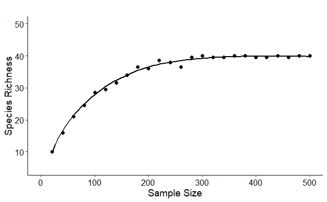
Species Richness vs. Sample Size. A graph showing the number of species as a function of sample size. On the left, the steep slope of the curve indicates that a large portion of the species richness is yet to be discovered. As the curve flattens toward the right, it indicates that a sufficient number of individuals has been collected; additional sampling is unlikely to yield many more species. Figure by Matthew J. Pruden.
Sieve Size:
Sieve size can affect both sample size (number of taxa and individuals) as well as the degree of live-dead mismatch. Fine sieve sizes (≤ 1mm) are often dominated by juveniles, which are poorly preserved in death assemblages. In contrast, the use of coarse sieve sizes (> 5mm) may omit key species or species traits and lead to reduced sample sizes, thereby reducing statistical power. Sieve sizes of 1 - 2mm have the greatest live-dead match because they retain adult individuals and potentially key species (Kidwell 2013).
Analytical Comparisons
Nearly any method used to describe the living assemblage can be applied to the death assemblage, allowing for them to be compared to each other. Therefore, which method is used depends on the scientific question. For example: 1) Has species diversity changed between the living and death assemblages? 2) Has the ecological composition changed? or 3) Has the condition (e.g., health) of the molluscan community, improved, worsened, or stayed the same when comparing the death assemblage to the living assemblage?
To answer the first question, a researcher could calculate and compare the species richness (the number of unique species within an assemblage), and species evenness (a measure of the relative abundance of species), or they could use a variety of species diversity indices (Box 2). The second question focuses on how organisms interact with one another and their environment. For example, a researcher could assess changes in functional traits (e.g., feeding, mobility, size), such as calculating and comparing the relative abundance of species that filter food from the water (suspension feeders) versus species that sift food from the sediment (deposit feeders). To determine whether the condition of the community has changed for the third question, a researcher could measure the relative abundance of pollution-tolerant to pollution-sensitive species using metrics known as biotic indices. See Box 2 for more examples of different metrics and methods that conservation paleobiologists use to compare living and death assemblages.
Box 2. Examples of metrics for comparing living and death assemblages.
Community Structure
Richness - A measure of the number of unique species within a sample. When assessing the faithfulness of death assemblage (DA) species richness with respect to the living assemblage (LA), richness can be further broken down into the number of species only found in the DA, only found in the LA, or the number of species found in both.
Evenness - A measure of how equally distributed abundance is among species. A perfectly even community would be composed of species with equal abundance.
Common evenness metrics include: Hulbert’s PIE (Probability of Interspecific Encounter) index and Pielou’s evenness index. Both PIE and Pielou’s index values range from 0 (species abundances are all different) to 1 (perfect evenness).
Diversity - Diversity metrics combine both species richness and evenness into a single number. Often, the greater the diversity, the greater the species richness and evenness are. Common diversity metrics include: Shannon-Wiener Index, Simpson Index, and Effective Hill Numbers.
Community Composition
Taxonomic similarity - A measure of how many species are shared between the LA and the DA. The Chao-Jaccard index is a commonly used metric for measuring taxonomic similarity and ranges from 0 (none of the species are shared between the assemblages) to 1 (both assemblages are comprised of the same species).
Rank abundance - A ranking of species within the LA and DA from the most abundant to the least abundant. Rank abundance can be used to assess whether the two assemblages have the same dominant species. A common metric for rank abundance is the Spearman correlation, which can take values that range from -1 (species are ranked in opposite order) to +1 (species are ranked in identical order).
Biological Traits
Size-frequency Distribution (SFD) - The distribution of body sizes of an organism can provide both biological and taphonomic information. For example, if a LA SFD is right-skewed, it could indicate that the assemblage is dominated by small-bodied individuals, potentially juveniles depending on the species present. If a DA SFD is left-skewed, it could indicate a taphonomic loss of smaller individuals.
Feeding modes - Feeding modes describe the diet and feeding method of an organism. Common molluscan feeding modes include:
- Predator: Feeds upon, and actively hunts, prey.
- Browsing Carnivores / Parasites: Feeds on animals without killing them.
- Herbivore: Feeds on living plants / algae.
- Suspension feeder: Feeds on suspended particles in the water column.
- Deposit feeder: Feeds on particles on/within the seafloor sediment.
- Detritivore: Feeds on dead organic matter.
- Chemosymbiotic: Obtains energy from a symbiotic association with bacteria living in their tissue.
Biotic Indices
Biotic indices aim to numerically describe the condition, or health, of a biotic community using a variety of metrics, such as richness, diversity, biological traits, and the relative abundances of pollution tolerant to sensitive species. Common biotic indices include: AZTI’s Marine Biotic Index (AMBI), Multivariate-AMBI (M-AMBI), and Benthic Index (BENTIX).
References & Further Reading:
Dietl, G.P., Kidwell, S.M., Brenner, M., Burney, D.A., Flessa, K.W., Jackson, S.T., and P.L. Koch. (2015). Conservation paleobiology: Leveraging knowledge of the past to inform conservation and restoration. Annual Reviews of Earth and Planetary Science, 43: 79-103.
Kidwell, S. M., G. P. Dietl, and K. W. Flessa. 2009. Evaluating human modification of shallow marine ecosystems: mismatch in composition of molluscan living and time-averaged death assemblages. Paleontological Society Papers, 15: 113-139.
Kidwell, S. M. 2013. Time‐averaging and fidelity of modern death assemblages: building a taphonomic foundation for conservation palaeobiology. Palaeontology, 56(3): 487-522.
Wijsman, J.W.M., Craeymeersch, J.A., and P.M.J. Herman. 2022. Comparing grab and dredge sampling for shoreface benthos using ten years of monitoring data from the Sand Motor mega nourishment. Journal of Sea Research, 188: 102259.